2.3.1. Energy uptake, assimilation and mobilization

For an individual in school \(i\), the energy uptake from food at time step \(t\) is described by a Holling’s type 1 functional response \(f\) (Holling [1959]) that depends on its somatic mass \(w(i, t)\) (Christensen and Walters [2004], Holt and Jørgensen [2014], Shin and Cury [2004]) in two ways.

First, it determines prey food biomass \(P(i,t)\) available to an individual of school \(i\) from the other schools and lower trophic levels present in the same grid cell \(c(i,t)\) according to a minimum \(R_{min}(s(i))\) and a maximum \(R_{max}(s(i))\) predator to prey size ratio (Shin and Cury [2004], Travers et al. [2009]):

\[P(i,t) = \dfrac{\sum_j{ \gamma(s(i), s(j)) B(j, t)}}{N(i, t)}\]

with

\[j \in \left( j \lor (c(j,t)=c(i,t)) \left( \dfrac{L(i,t)}{R_{max}(i)} \leq L(j, t) \leq \dfrac{L(i,t)}{R_{min}(i)} \right) \right)\]

where \(\gamma(s(i), s(j))\) is the accessibility coefficient essentially determined by the position of potential prey schools \(j\) in the water column relative to that of school \(i\) and \(B(j,t) = N(j,t) w(j, t)\) is the biomass of prey school \(j\) . Second, it sets the maximum possible ingestion rate according to an allometric function with a scaling exponent \(\beta\). The energy uptake can then be written as:

\[I(i,t) = f(P(i,t)) = min(P(i,t); I_{max}(i) \psi(i, t) w(i,t) ^{\beta}\]

with \(I_{max}(i)\) the maximum ingestion rate per mass unit at exponent \(\beta\) (or mass-specific maximum ingestion rate) of individuals in school \(i\) and \(\psi(i,t)\) a multiplicative factor that depends of their life stage according to:

\[\psi(i, t) = \Biggl \{ { \theta \text{ if } a(i,t) < a_l \atop 1\text{ otherwise } }\]

where \(a_l\) is age at the end of a fast growth period (e.g larval period or the larval and post-larval period) and \(\theta\) a factor accounting for higher mass-specific maximum ingestion rate at this stage. A portion \(\xi\) of the energy uptake \(I(i,t)\) is assimilated, a fraction \(1 - \xi\) being lost due to excretion and faeces egestion.

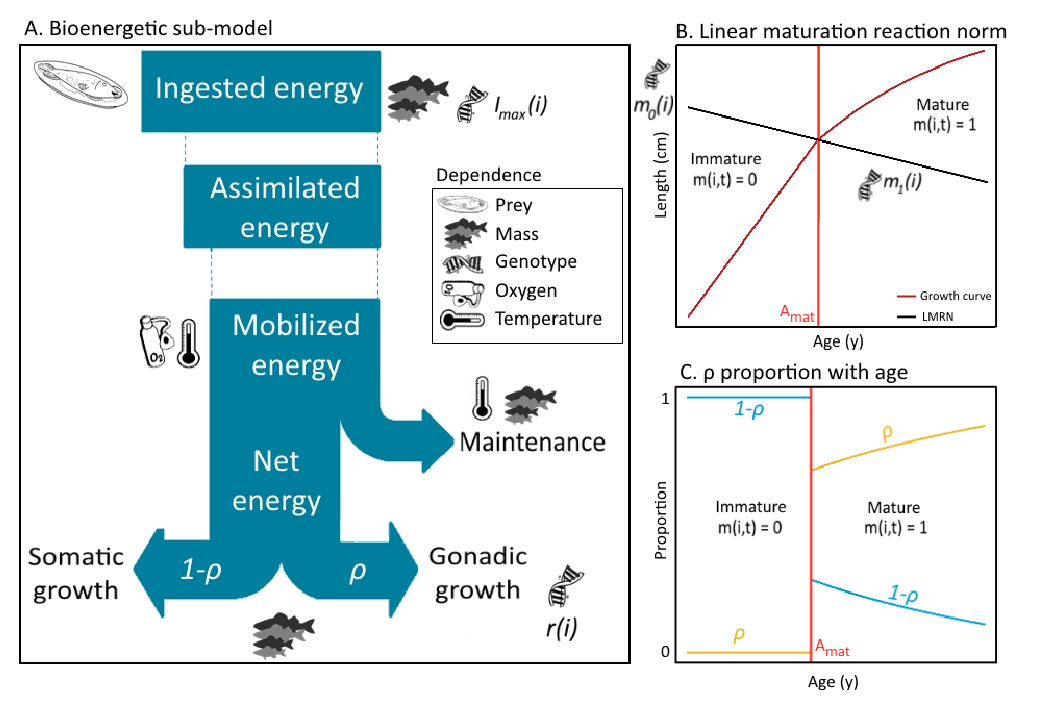
Fig. 2.1 Summary of the processes at stake in the Bioen-OSMOSE version.

No reserves are modeled in EV-OSMOSE, hence all the assimilated energy can be directly mobilized. Mobilized energy \(E_M\) , referred to as active metabolic rate in the ecophysiology literature, fuels all metabolic processes such as maintenance, digestion, foraging, somatic growth, gonadic growth, etc… The mobilization of energy relies on the use of oxygen to transform the energy held in the chemical bonds of nutrients into a usable form, namely ATP [Clarke, 2019]. In consequence, the maximum possible energy mobilized at a given temperature depends directly on dissolved oxygen saturation and, as temperature increases, on the capacity of individuals to sustain oxygen uptake and delivery for ATP production (see section 1.2.1 Basic principles for more details). The mobilized energy rate \(E_M\) is thus described by

\[E_M(i,t) = \xi I(i,t) \lambda \left([O_2](i, t)\right) \varphi_M(T(i, t))\]

with \(\lambda \left([O_2](i, t)\right)\) and \(\phi_M(T(i, t))\) being the mobilization responses to dissolved oxygen saturation and temperature encountered by school \(i\) in the grid cell it occupies at time \(t\) . These are scaled between 0 and 1 such that, in optimal conditions, all assimilated energy \(E_M(i,t) = \xi I(i, t)\) can be mobilized and, in suboptimal conditions, only a fraction of assimilated energy can be mobilized (\(E_M(i,t) < \xi I(i, t)\)). More precisely, the effect of dissolved oxygen is described by a dose-response function \(\lambda\) [Thomas et al., 2019] which increases with the saturation of dissolved oxygen:

\[\lambda([O_2]) = C_{O,1} \dfrac{[O_2]}{[O_2] + C_{O, 2}}\]

with \(C_{O,1}\) and \(C_{O, 2}\) the asymptote and the slope of the dose-response function.

The effect of temperature is described according to the Johnson and Lewin [1946] model [Pawar et al., 2015]:

\[\varphi_{M}(T) = \Phi \dfrac {e^{\dfrac{-\varepsilon{}_M}{k_BT}}} {1 + \dfrac{\varepsilon_M}{\varepsilon{}_D - \varepsilon{}_M} e^{\dfrac{\varepsilon{}_D}{k_B}\left(\dfrac{1}{T_P} - \dfrac{1}{T}\right)} }\]

with \(k_B\) the Boltzmann constant, \(\varepsilon_M\) the activation energy for the Arrhenius-like increase in mobilized energy with temperature \(T\) before reaching its peak value at \(T_P\) , \(\varepsilon_D\) the activation energy for the energy mobilization decline with \(T\) after \(T_P\) , and

\[\Phi = \left(1 + \dfrac{\varepsilon_M}{\varepsilon{}_D - \varepsilon{}_M}\right) {e^{\dfrac{\varepsilon{}_M}{k_BT}}}\]

a standardizing constant insuring that \(\psi_M(T_P) = 1\).

The thermal responses of the bioenergetic fluxes is summarized in Fig. 2.2

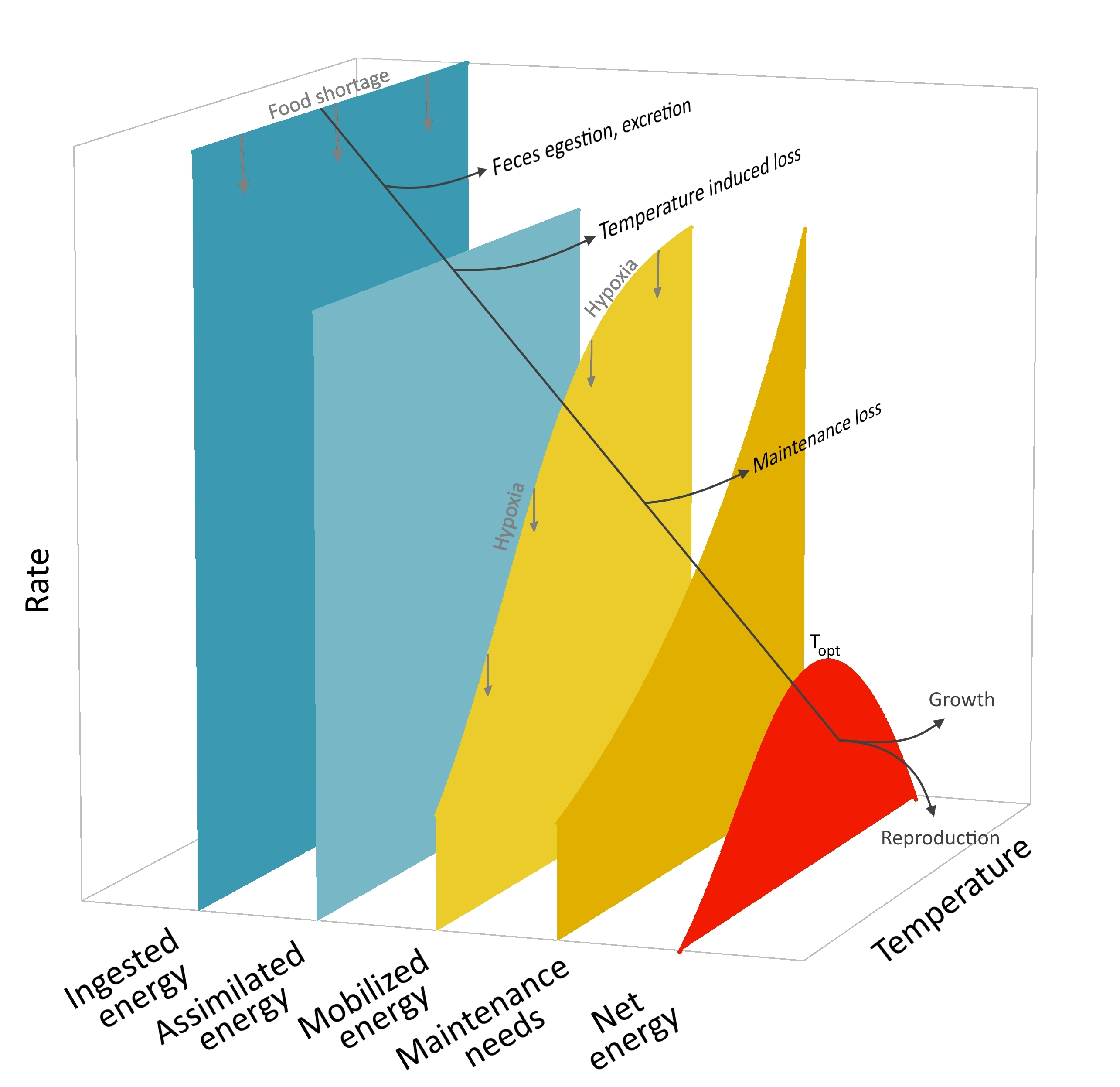
Fig. 2.2 Thermal responses of the bioenergetic fluxes from ingestion to tissue growth in Bioen-OSMOSE. The net energy rate dome-shaped curve (in red) conforms to the OCLTT theory and the principle of TPC. Food shortage impacts ingested energy and downstream fluxes. Hypoxia impacts mobilized energy and downstream fluxes. The maximum of the net energy rate (red curve) is called \(T_{opt}\) hereafter.