7.2. Reading Osmose parameters
The loading of Osmose parameters is achieved by using the read_osmose function with an input argument providing the path of the
main configuration file.
suppressMessages(require("osmose"))

output.dir = file.path("rosmose", "_static")

exampleFolder <- tempdir()
demoPaths <- osmose_demo(path = exampleFolder, config = "eec_4.3.0")

# load the Osmose configuration file
osmConf = readOsmoseConfiguration(demoPaths$config_file)

# Summarize the configuration
summary(osmConf)

# extracting a particular configuration object
sim = get_var(osmConf, what="simulation")

# proper way to recover the season parameter (returns a vector of numeric)
movements = get_var(osmConf, what='movement')

# Plotting reproduction growth
png(filename = file.path(output.dir, 'species.png'))
plot(osmConf, what="species", species=0)

# Plotting reproduction seasonality
png(filename = file.path(output.dir, 'reproduction.png'))
plot(osmConf, what="reproduction", species=1)

# Plotting size range for predation
             Length Class  Mode
osmose        2     -none- list
mortality     4     -none- list
simulation    7     -none- list
fishing       1     -none- list
movement      7     -none- list
fisheries     9     -none- list
predation     4     -none- list
reproduction  1     -none- list
species      17     -none- list
grid          3     -none- list
population    1     -none- list
output       19     -none- list
Furthermore, some parameters can be plotted for a given species. This is done as follows:
png(filename = file.path(output.dir, 'predation.png'))
plot(osmConf, what="predation", species=2)
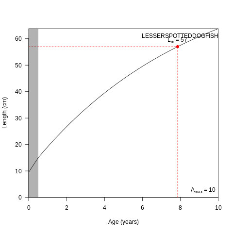
Fig. 7.1 Growth parameters for species 0
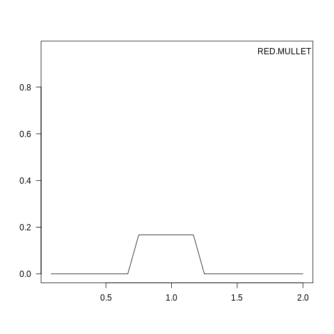
Fig. 7.2 Reproduction seasonality for species 1
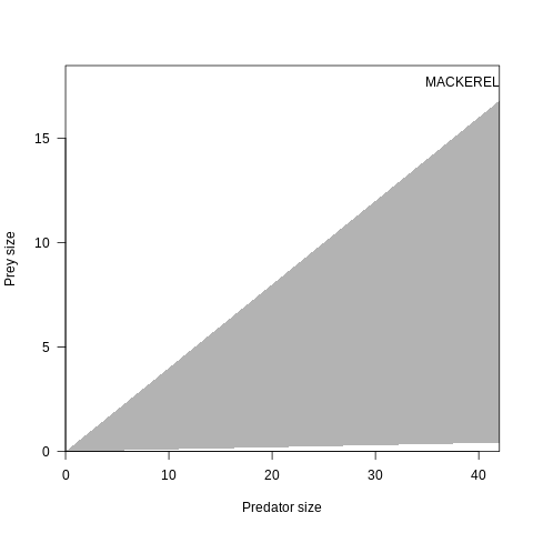
Fig. 7.3 Predation size range for species 2