7.5. Plotting outputs
Plotting Osmose outputs is achieved by calling the generic plot function on the osmose object, output by the read_osmose function. The function takes as argument the variable to be displayed (what argument).
The species argument allows to specify the indexes of the species to display (cf. the X in the species.name.spX parameters).
library("osmose")

input.dir = file.path("eec_4.3.0", "output-PAPIER-trophic")
data = read_osmose(input.dir)

output.dir = file.path("rosmose", "_static")

test = get_var(data, "species")

png(file=file.path(output.dir, "biomass.png"))
plot(data, what="biomass")

png(file=file.path(output.dir, "abundance.png"))
plot(data, what="abundance", species=c(0, 1, 2))

png(file=file.path(output.dir, "yield.png"))
plot(data, what="yield")

png(file=file.path(output.dir, "yieldN.png"))
plot(data, what="yieldN")
Hint
When several replicates are run, the uncertainty due to the stochastic mortality is displayed as a grey shading.
Warning
At this time, only these four variables can be plotted. However, more plot functions (diet matrix, mortality, etc.) will be released soon.
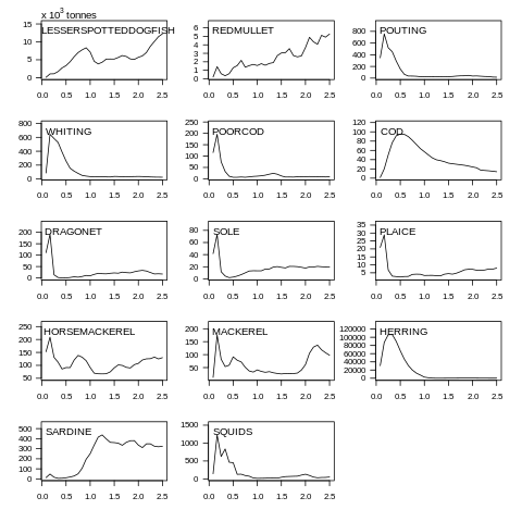
Fig. 7.4 Biomass plot
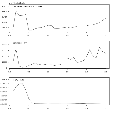
Fig. 7.5 Abundance plot
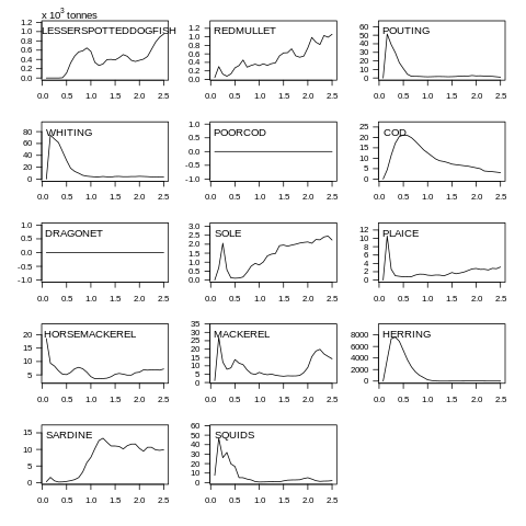
Fig. 7.6 Yield biomass plot
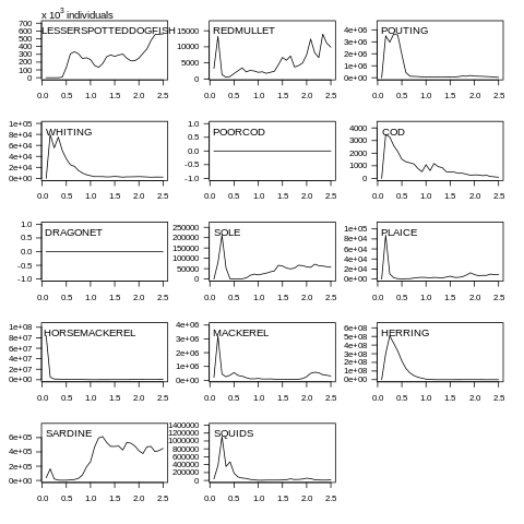
Fig. 7.7 Yield abundance plot